Computational Complexity - Solving Real Life Problems

Computational Complexity is a measure of the computational time taken by a particular algorithm. In a scenario where there are multiple algorithms available for a particular problem, the effectiveness of any particular algorithm is gauged on the basis of the time constraint. This is done by breaking the algorithm into its basic steps and then taking a count of each of them. Hence greater is the number of steps, greater is the complexity. Now for example, if we take two 5 bit binary numbers and XOR them, the number of steps taken is 5 and if the same process is repeated for a 100 bit binary number, the number of steps goes up to 100. The algorithm employed in either case is the same; the complexity is given by the size of the numbers.

When we say size of a number n, it is defined as the number of binary bits which are required to denote ‘n’ in base 2. For example, 5 in base 10 when expressed in binary takes the form 101, thereby giving n = 3. Similarly 20 is given by 10100₂ which makes n = 5. Now if we XOR any two numbers each of size n=b, the number of steps taken will be ‘b’. Hence we can say that XORing those numbers has computational complexity of order ‘b’ which is denoted by O(b). This can be applied to even simpler applications like addition wherein if we are to add two n digit numbers, the minimum number of steps taken (ignoring any carry over from the previous step) will be equal to n as we approach from right to left. This can’t be avoided because we need to know every number before we can add them. Coming back to the XOR example stated above, if we are to double the size of the numbers, we will end up doubling the size of the steps required hence increasing the time needed. One important point to take into consideration is that computational complexity is not dependent on the capacity of the machine or in other words, it is independent of implementation. This factor becomes important because different machines may take different times `while processing the same ‘b’ basic steps. Another important point to consider is that for any algorithm with computational complexity defined as O(b), if we are to multiply the size of the problem by X,  the computational time will have the same effect of being multiplied by X as well.

Image Courtesy: freedigitalphotos.net, ddpavumba

Big O notation is used to describe the asymptotic behavior of the functions in complexity theory. It tells you at what rate will the function grow. Rate at which a function grows is called order, hence letter O is used as its notation. Let f(x) and g(x) be two functions defined in real numbers. Then the big O notation would be represented as:

f(x) = O(g(x)) (for x belonging to real numbers) if and only if there exist certain constants N and C such that

|f(x)| <= C|g(x)| for all x>N

Basically it means that our function cannot grow faster than the function defining its time dependence complexity.

Commonly used functions as g(x) to describe time dependence are as follows written in increasing order of their growth rate (c is some constant)

O(1) constant

O(log(n)) logarithmic

O((log(n))^c) polylogarithmic

O(n) linear

O(n²) quadratic

O(n^c) polynomial

O(cⁿ) exponential

As explained above, when it comes to addition, the complexity of adding two binary numbers is given as O(b). However if we are to multiply those numbers, the complexity changes to O(b²). We can take a simple example to illustrate this change. Let’s say we are to multiply two numbers 34 and 56. This will involve multiplication in 4 basic steps and then making carry over adjustments accordingly to get the final result. Hence the complexity for this case becomes O(2²). Similarly, if we double the bit size of the numbers to be multiplied, the time required changes to O[(2b)²] = O(4b²).

So complexity theory basically classifies the problems on the basis of the difficulty faced in solving them.

This brings us to the concept of P and NP problems:

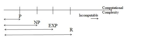
1. Deterministic Polynomial-Time (P) Type

A problem is basically classified as that belonging to the P (polynomial time) class if there is at least one algorithm which can solve that problem; the number of steps employed by the algorithm being restricted by a polynomial in ‘n’, where n gives the length of the input used.

An algorithm, existing or newly created is said to abide by polynomial time if, for a given input, the number of steps essential to complete the algorithm is given by O(n^k) for some nonnegative integer k, where k gives the complexity of the input provided. Algorithms using polynomial-time are considered to be fast, feasible and efficient. A large number of day to day mathematical applications such as addition, subtraction, multiplication, and division in addition to square roots, logarithms and powers can be performed using polynomial time.

A specific term which comes into being in the deterministic approach is the time complexity of an algorithm. It measures the time taken by any algorithm as a function of the length of the string representing the input provided by the user or any other source.

Time complexity of an algorithm is normally expressed using the Big O notation, as already mentioned above. It does away with all the coefficients and other lower order terms. When an algorithm is expressed in this fashion, we can say that its time complexity has been described asymptotically i.e. its input size has the freedom to approach infinity. To illustrate this point, we can take the help of an algorithm where the time required for all inputs of size n is at most 5n³ + 3n. Hence, the asymptotic time complexity for this algorithm is O(n³)

A few examples of polynomial time algorithms that we find in everyday usage have been given below:

• In computer science, the quick sort algorithm when applied on n integers performs at the maximum Cn² number of operations for a given constant C. Thus the running time is represented by O(n²) which makes it a polynomial time algorithm.
• Also as illustrated above, arithmetic operations of the likes of addition, subtraction, multiplication, division et al can be expressed in polynomial time

2. Non Deterministic Polynomial-Time(NP) Type

An NP problem is one which has a solution, inputs to the solution and a verifier which runs in polynomial time. The verifier has to take both the inputs and their corresponding solution into consideration and tell the user whether they are in sync.

NP essentially consists of the set of all decision problems wherein the state of the problem, whether ‘yes’ or ‘no’ has to be supported by efficiently verifiable proofs that it is indeed so. Effectively, these proofs will have to be validated in polynomial time with the aid of a deterministic Turing machine. Defined equivalently in a more formal fashion, NP represents the collection of all such decision problems where the "yes" instances have been accepted in polynomial time by a non-deterministic Turing machine. To gauge the equivalency of the two definitions stated above, we can refer to the fact that an algorithm on such a non-deterministic machine as a Turing machine is divided into two phases - the first phase involves making the nearest possible guess about the solution, which is again generated in a non-deterministic fashion; the second phase makes use of a deterministic algorithm that does the job of verifying or rejecting the guess as made above, as a valid resolution to the current problem

A fantastic example of non deterministic problem solving comes from ‘factoring’ wherein one needs to decide the factors (say a*b=N) of a particular large number N barring the number itself and 1. Theoretical analysts have observed it time and again that if we are to take two numbers of one thousand digits each and multiply them together in a computer, it takes hardly a few seconds to arrive at the result while if we feed this very output to the computer again to get it decomposed into factors, it’s possible that the computer may not figure out an efficient solution for millions of years. This raises the question as to why we need to go through so much of distress to arrive at factors of such a large number. And the answer, as it turns out is of paramount importance with a potential to change the state of an economy. Let’s say one of our friends wants to impersonate a bank. And unlike years back, when the transaction between banks happened in the form of gold bricks transported in trucks, the transactions now are done via online funds transfer through severely protected connections. As it turns out, the encryption algorithm they use to secure their transactions is called RSA. In RSA, each party has a secret key that consists of two numbers p & q – big prime numbers and then they have a public key say n which is equal to p*q. This public key is released to all so that other people are able to send messages via this network, which in turn will be decrypted by the partnering parties using the public key. Now let’s say our friend wants to intervene here. He is in charge of an efficient verifier which is capable of performing large divisions. He has n and then he obtains a P_guess which gives n% P_guess =0

3. Exponential Problems

EXP refers to the set of problems that can be solved in exponential time. Exponential time algorithm is the one in which time is upper bounded by 2poly(n), where poly(n) is a polynomial in n. ie the T(n) is bounded by O(2^nk) for some constant k. For eg. N*n chess board problem is EXP type of problem. It cannot be solved in polynomial time.

R refers to problems that can be solved in finite them. These are the problems are basically solvable. R refers to recursive function. The problems can be solved by recursive algorithms in finite time belong to this category. However solvable problems represent a very small part of the problems available with us. The rest of the problems are mathematically unsolvable.

Complexity Analysis of the real life problems:

Step 1: To apply computational complexity in real life, we first need to convert the real life problems into a yes-no problem without altering its complexity. A threshold value in the input is needed for the conversion. The problems are generally of two types- feasibility or satisfice problems. For eg. Scheduling a production facility, timelines and deadlines of the production process and scheduling without delay in jobs. A certain standard examples of real life instances are presented below:

One-Machine Deadline Scheduling Instance: Here we are scheduling the machine operation wrt to its processing time feasibility so that deadlines are met.

Let the processing times be defined as ti and deadlines for the jobs be di where i varies from 1 to n.

Then our problem can be represented as:

Question: Do we have a set of start times si>0 for  i varying from 1 to n such that sj does to belong to the set [si, si+ti) where i≠j so that one start time does not clash with another start time under the constraint that it meets the deadlines for each task si+ti <= di ?

Two-Machine Line Balancing Instance: Our task here is to divide the jobs between two machines K and J, evenly when the processing time are known. It can be represented as follows:

Let the set of processing times be ti where i varies from 1 to n. Let there exist a number v

Question: Can we divide the indices i =1 to n such that difference between the time taken by the processes on machine K and the time taken by the processes on machine J be less than or equal to v.

A more restricted version of above problem would be when a perfect balance is required ie v=0.

Then the question would be: Can we divide the indices i =1 to n such that the time taken by the processes on machine K is equal to the time taken by the processes on machine J.

This equal time problem is called two partition problem. This problem is harder to deal with than the two machine line balancing because it is more restricted

Step 2: So the next step we need to understand is how to find the complexity of any problem. So some basic things that contribute to making a problem hard are as follows: when a perfect division of resources is required, sequencing decisions which consider both where you currently are and where you were before, splitting into subsets a set of objects where there exists a constraint for each subset, to find out the largest substructure which satisfies a property, minimizing or maximizing unions and intersections of sets. Substituting the threshold value with a restricted value may also sometimes alter its complexity. So we need to be very careful in doing so. It is important to figure out what makes the problem hard, it may be difficult to get balance fit. Two partition is an example of it. On the other hand, it can be easy for a problem to balance everything but hard to minimize the negative effects of not obtaining the perfect combination. Independent set which requires a maximum size set of vertices of a polygon such that no two of them are connected by an edge is an example of second type. Hence, Identify the type and work accordingly.

As we solve more number of problems, we develop an intuitive ability to recognize the hard part of the problem. Let’s see how to identify a NP hard problem. First identify a hard problem and then think of a easy problem to contrast it. Compare both the problems and identify what makes the hard problem easy. Some examples of constraints are as follows:

Integer Programming (IP) : Maximise c*x subject to a constraint of Ax<=b where x is an integer.

Contrast: Linear programming is easy and so is Integer programming when the constraints have one of two dimensions fixed (unimodular). Dimensions here refer to the no. of variables and total constraints.

Two-machine weighted flow-time minimization: Given two parallel processors and a set of jobs with individual processing times and weights, find a schedule to minimize the weighted sum of completion times.

Contrast: If the given weights or the times are equal then the problem will be easy for any no. of processors. Run equal weights or equal processors constraint one at a time.

Steiner tree: Given a graph G = (V, E), edge lengths, and a subset S of vertices V, find a tree in G of minimum total length that contains S. (The tree may contain vertices in V - S; try connecting the vertices of a square in the plane.)

Contrast: The minimum spanning tree problem, in which S =V, is easy.

Normally the hard problems can be solved with dynamic programming. If dynamic programming does not help then other methods like off the shelf mathematical software’s or heavy-duty mathematical programming methods and heuristics can help.

Easy problems can be solved using linear programming, simplex methods and integer programming etc.

Reductions:

In computational complexity, reduction is defined as transforming one type of problem into another. A problem X is reducible to problem Y if X’s algorithm can be used to solve Y too. This means that problem Y is easier to solve than X. There are two types of reductions that we use: many-one reduction and the Turing reduction. A many to one reduction is done by mapping instances of a problem into the instances of other problem. Turing reduction on the other hand works by solving one problem assuming that the other problem is easy. Turing reduction is stronger than many-one reduction. However, stronger reductions are not effective in separating problems though they are easier to design.

Reductions are useful when they are easy. Take for instance, a difficult NP-complete problem can be reduced to a trivial problem. Also, it can convert an incomputable problem to a decidable one. Reduction is used in problems like halting problem to prove that language is not decidable ie the turing machine M would halt when input of string w is given(H(M,w)). This language is said to undecidable. Now if F(M) is the problem of determining the whether the input language to the turing machines is empty or not then we know by reduction from H that F is undecidable.

Conclusion:

Basic understanding of computational complexity helps a manager to determine the time he would take to solve the real life problem at hand and judge how large the instance of problem actually is. Also, choice of algorithm is more important than the choice of hardware and data structures. Classifying the problems as easy of NP-hard will tell us the available methods to solve it. Deciding the final method can then be done looking at other aspects also like size, financial stake, desirable accuracy and time constraints. Computational complexity is an ineluctable phenomenon. Most problems are hard to solve. But realistic cases are almost easy every time if we study them hard enough. As a manager, the basic learning and application of computational complexity helps us majorly in problems related to operations. As in the above text certain examples like machines scheduling, meeting deadlines, minimizing late jobs have been cited, similarly we can use it for problems in our production facility and reduce the time to solve by using appropriate methods available for a particular type of complexity.

This article has been authored by Pooja Punjabi and Manash Hazarika from IIM Kozhikode

REFERENCES:

• http://en.wikipedia.org/wiki/Computational_complexity_theory
• http://theory.stanford.edu/~trevisan/notes/complexitynotes02.pdf
• http://www2.isye.gatech.edu/~ctovey/tovey.tutorial.pdf
• http://staff.science.uva.nl/~ulle/teaching/comsoc/2012/slides/comsoc-complexity-tutorial.pdf